Maximum Likelihood for Fitting Models

Let’s take a very abstract look at what we want to do when we “fit” a machine learning model.

For our purposes, a model is a big mathematical equation with an input and output and a preset number of “knobs” or parameters we can twist to change the equation’s behavior in predetermined ways. A simple model might be a line—a linear model; the parameters would be the slope and intercept.

In most cases we have a model we want to use for a certain task but have no idea what the parameter values (knob settings) should be to get it to actually do the task. Maybe I want to use the number of runs a baseball team scores over a season (the input) to linearly estimate the number of wins they had in that season (the output):

\[\underbrace{y}_{\text{wins}} = m\cdot\underbrace{x}_{\text{runs}} + b\]

However, I don’t know what slope $m$ and intercept $b$ values actually capture this relationship.

Machine learning solves this problem. Machine learning refers to the algorithms we use to figure out how to configure the knobs on our model based on observed data. That’s it. No magic, just math (as we’ll see). These algorithms follow a series of steps designed to estimate the parameter values required to make the model line up with the observed data.

The dataset describes our problem empirically—implicitly through a set of unstructured observations. This becomes handy when we struggle to define our task theoretically—explicitly through an equation or other structured form. Here’s a few examples to illustrate the difference:

Task	Theoretical/Explicit/Structured	Empirical/Implicit/Unstructured
Playing tic-tac-toe	The rules of tic-tac-toe	Examples of many tic-tac-toe games
Predicting how an object falls	The physics equations that calculate the position of an object as it falls	Many high-speed videos that show objects falling
Identifying bears	Words that describe what a bear looks like	A bunch of bear pictures
Recognizing a song	Written sheet music	An audio recording
Predicting a baseball team’s wins using their total runs scored	???!	The number of runs and wins from many different teams

Inferring Parameters from Data

If you think about it, each example in the dataset contains information about the parameters. We want to extract this information through inference. Just like knowing you’re drinking hot cocoa tells us something about whether it’s snowing, knowing that we are working in a world where data point ($x$ runs, $y$ wins) was observed tells us something about the range of likely values for model parameters $m$ and $b$. If we say that $\theta$ represents the knob settings or parameters (the slope and intercept in this case), then we want to infer $p(\theta \mid x)$—the likely values for the parameters given (“conditioned on”) the observed data point.

The “best” slope and intercept are those that maximize the inferred probability. These are the most likely parameters given the observation. We can break down the inference using Bayes’ Rule:

\[\begin{equation} p(\theta \mid x) = \frac{p(x \mid \theta)p(\theta)}{p(x)} \end{equation}\]

In the hot cocoa example, we saw that the denominator is a scaling factor that rescales the chance for worlds where $x$ actually happened. Unfortunately, $p(x)$ is “intractable” in general, meaning that we can’t efficiently measure or calculate it. Thankfully, we actually don’t care about the precise value of $p(\theta \mid x)$; we are just trying to find the parameters that cause the maximum value. That means we can safely multiply this inferred distribution by any constant scaling factor. The maximum value itself will change, but it will occur for the same parameters.

If we use a uniform prior $p(\theta) = \text{constant}$ and recognize the $p(x)$ will have the same value for any specific $x$, we can remove these factors and see that the inferred posterior distribution is proportional to something we call the “likelihood function”:

\[\begin{equation} p(\theta \mid x) \propto p(x \mid \theta) \end{equation}\]

The likelihood function tells us how likely some data point is given specific knob settings (parameter values). A simple likelihood function would be 1 if the data exactly matches the model’s output with those parameters and 0 otherwise. For our baseball example, this might look like:

\[p((x, y) \mid m, b) = \begin{cases} 1, &\text{if } y = mx + b \\ 0, &\text{otherwise} \end{cases}\]

If we fix the $x$ runs and $y$ wins values to one of our data points, we can see how this likelihood changes for various values of the slope and intercept: For example, the 2023 Texas Rangers scored 881 runs and won 90 games. If we plug this in for $x$ and $y$ in our model, we get

\[p((881, 90) \mid m, b) = \begin{cases} 1, &\text{if } 90 = m(881) + b \\ 0, &\text{otherwise} \end{cases}\]

There are certain values of $m$ and $b$ that make this equation true. Those are the parameters that make our model match this data point. We can actually plot these valid combinations as a line:

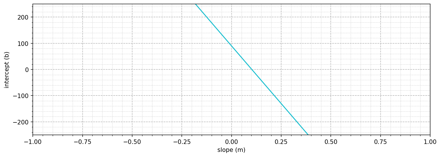
All of these possible solutions are equally valid because they all have the same likelihood score of 1 and predict the correct wins from the runs. We can repeat this for all the data points:

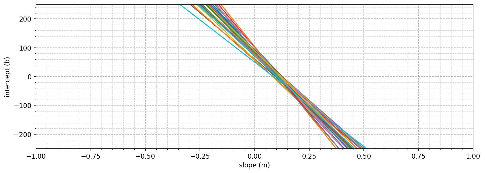
The “perfect” solution would be one where all the lines intersect. We can create a combined or joint likelihood function for all the points by multiplying the individual likelihood functions together. Each function is either 0 or 1. The product of all of them will only be 1 if every factor is also 1, meaning every data point is exactly matched:

\[\begin{aligned} p(x^{(1)}, x^{(2)}, \dots, x^{(N)} \mid \theta) &= p(x^{(1)} \mid \theta)p(x^{(2)} \mid \theta)\cdots p(x^{(N)} \mid \theta) \\ &= \prod_{i=1}^{N} p(x^{(i)} \mid \theta) \end{aligned}\]

However, because the relationship isn’t perfect—teams could have similar run totals but different win totals—this perfect point doesn’t exist.

We can fix this by relaxing our draconian likelihood function. Instead of demanding an exact match to every data point, we can make each line a smoother “bump” around the exact fit line:

\[p((x, y) \mid m, b) = \exp \left(-\frac{(y - (mx + b))^2}{2 \sigma^2}\right)\]

This function takes the exponential of the squared error between the prediction $mx + b$ and the observed wins $y$. The $\sigma$ is a constant we pick for how relaxed the likelihood should be (bigger means more forgiving). Here’s what it looks like for the Rangers:

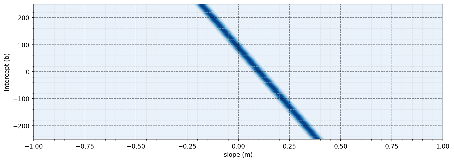
Notice that there is now a band of values that could work for our model. Just like before, we can multiply likelihoods of points together to get the combined likelihood. Here’s how it might look if we combined the Rangers and Rockies:

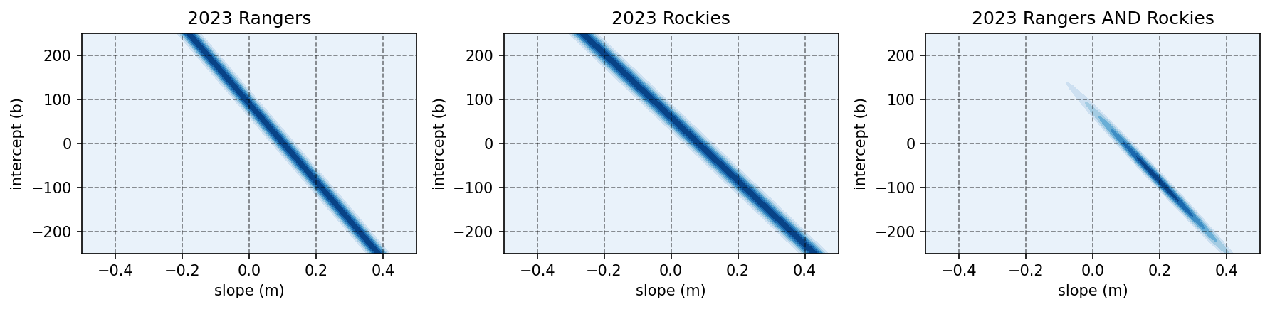
Notice how putting both together constrains the range of good combinations but still leaves a range of possible knob settings. You can imagine that as we multiply more and more likelihood functions together, we get a tighter and tighter bound around “good” combinations of slope and intercept. The parameters we pick at the peak of the final combined likelihood function are considered the “best” fit. Note that we don’t know how good of a fit this is—the predictions might actually be pretty bad— just that it’s the best we could find.

Maximizing the Log Likelihood

While straight maximizing the combined likelihood is conceptually what we want to do, it’s actually very hard computationally. If we multiply a bunch of factors together, the result can very quickly get close to zero. Computers can only be so accurate, so eventually the “close to zero” value gets rounded down to zero. Not good. Plus, multiplication is annoying/slower/harder when compared with a simpler operation like addition.

To make things easier, we can wrap everything in a logarithm and applying convenient properties. Like a constant scaling factor, putting everything inside a log function might change the height of the maximum peak, but it doesn’t change the location. Thus, maximizing the log likelihood gives us the same slope and intercept values as maximizing the likelihood:

\[\begin{equation} \begin{aligned} \hat \theta &= \underset{\theta}{\arg\max}\prod_{i=1}^N p(x^{(i)} \mid \theta) \\ &= \underset{\theta}{\arg\max}\log \left(\prod_{i=1}^N p(x^{(i)} \mid \theta)\right) \\ &= \underset{\theta}{\arg\max} \sum_{i=1}^N \log p(x^{(i)} \mid \theta) \\ \end{aligned} \end{equation}\]

If take this approach to sum up the log likelihoods of all our baseball data points, we get a plot that looks something like this:

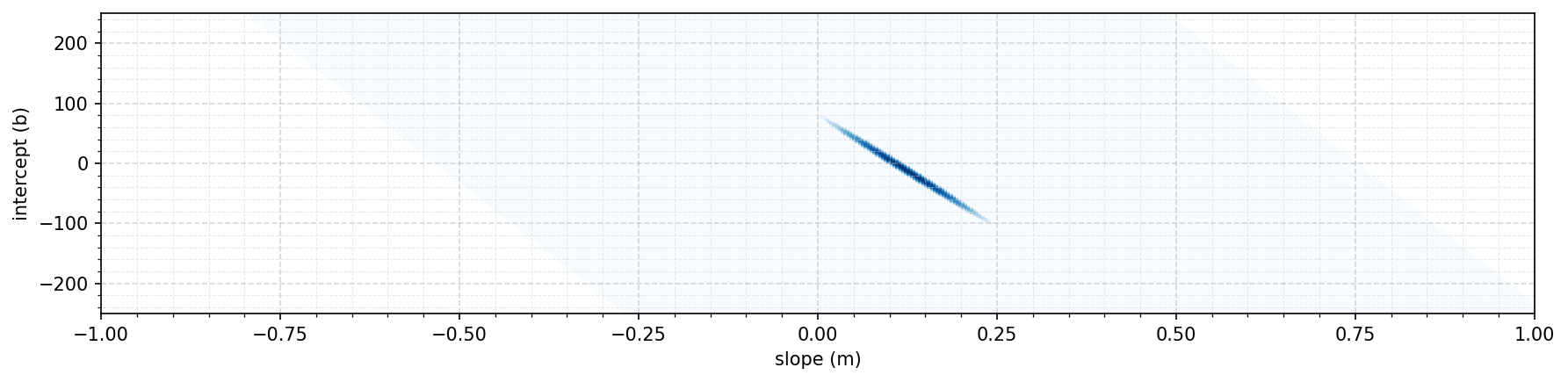
It turns out that this function has it’s maximum point when $m = 0.122$ and $b = -10.5$. Now we can put these into our model and plot the model line vs. the actual data points:

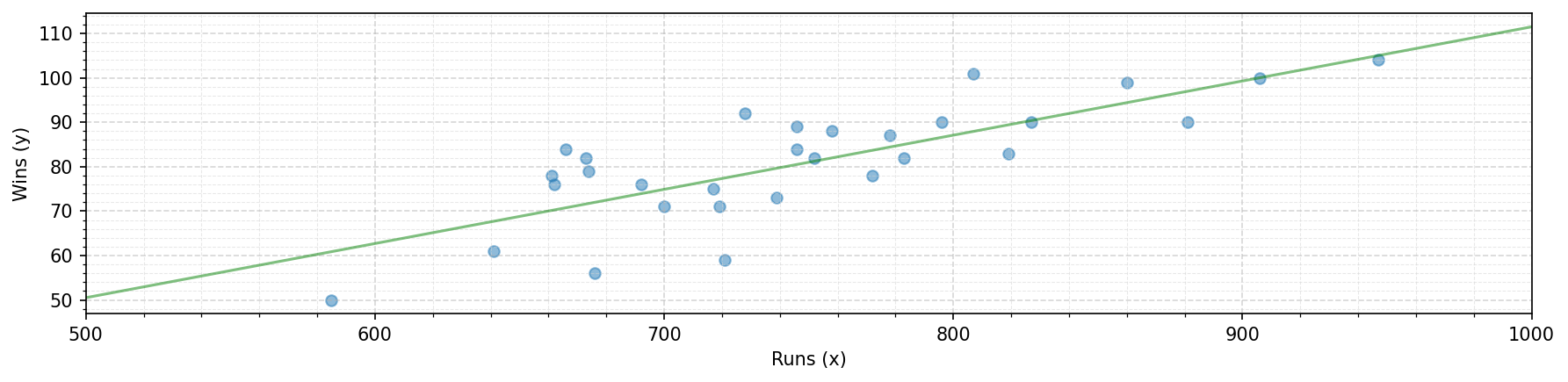
Not perfect, but it does look like a fairly reasonable linear fit for our task!

Minimizing the Expected Negative Log Likelihood

If we go back to equation (3), we can divide by the number of data points $N$ and make the log likelihood equation look like an average, or an expected value, recasting our problem as maximizing the expected log likelihood across the distribution of observed data points:

\[\begin{aligned} \hat \theta &= \underset{\theta}{\arg\max}\ \frac 1 N \sum_{i=1}^N \log p(x^{(i)} \mid \theta) \\ &= \underset{\theta}{\arg\max}\ \mathbb E_{p_\mathcal{D}(x)} \left[\log p(x \mid \theta)\right] \end{aligned}\]

Note that when we convert to an expectation, we have to specify the distribution that the data points come from (are sampled from). We use $p_\mathcal{D}(x)$ to represent the “empirical distribution” of observed data points.

Many optimization algorithms are designed to find the minimum point of a function. We can flip our likelihood with a negative sign to work with them since maximizing the log likelihood is the same as minimizing the the negative log likelihood.

\[\hat \theta = \underset{\theta}{\arg\min}\ {-\mathbb E}_{p_\mathcal{D}(x)}\left[ \log p(x \mid \theta)\right]\]

In one final notation switch, we often write $p(x \mid \theta)$ as $p_\theta(x)$, indicating that the likelihood is “parameterized” by the knobs $\theta$, distinguishing $\theta$ as parameters and not another input to the model:

\[\hat \theta = \underset{\theta}{\arg\min}\ {-\mathbb E}_{p_\mathcal{D}(x)}\left[ \log p_\theta(x)\right]\]