The Kalman Filter

Let’s say you’ve been going on more runs recently, and you want to track your mile pace. Obviously, you can find an average mile pace for each run by dividing the distance by your time. However, this could be noisy and unstable—on some days you might be sluggish while on others the perfect confluence of factors might set you up for a personal best. An alternative would be to average all your recorded mile times or do a running average of the last five. This would be better, but if you are steadily improving, the better times of your recent runs could be dragged down in the average by older, worse times. In general, the “hidden” information we want—your “true” mile time at this instant—is obscured by a variety of factors so we can’t measure it directly.

A solution might be to blend two sources of information. The mile times actually measured are noisy and variable, but they do contain some information about the true mile time that we want. On the other hand, we also know that it should improve slightly with each run. We’ll call the first source the “observation” and the second the “model.” We can cross-check the expected true mile time according to the model and the observed mile time to produce a better estimate of the true, hidden value.

How do we combine them? If the model’s output and the observation are different, how do we know which one to believe or in what proportion? The critical piece for solving this puzzle is capturing the uncertainty or variability of each source. If the model is more confident, we’ll rely more on its prediction. If the measurement is more confident, we’ll be more willing to revise the model’s prediction to consider the measured mile time.

In most cases, the uncertainty surrounding our measured value is relatively constant. We might know that the measured mile time often swings up or down by one minute. The uncertainty around the model’s prediction is a little trickier because it involves two things. First, while the model might expect the true mile time to improve by 2% every run, there could be some real variability in this improvement. That is, the true mile time itself could have some variance intrinsically. In the observation, the variation is due to factors related to how we measure the value—temperature, rain, energy level, etc. For the model, we are implying that the actual hidden value also has some randomness due to fluctuations in your biological processes. Two identical runs in identical conditions could affect your true mile time differently. While the model can’t predict this “process variance,” we can guess its magnitude.

However, a second factor also influences the model’s overall variance: the confidence in the value fed into the model! Since we don’t ever get the true mile time, this input value is our previous estimate of the true mile time. Even if we are very confident initially, using the model to recursively predict future values intuitively decreases the confidence in each successive estimate. If we continue to churn along into the future without comparing to real measurements, our confidence in the model’s output will continue to decline since we get farther and farther removed from any grounding in reality.

With all this in mind, we can create our filtering algorithm. We start with an initial guess about the true, hidden mile time. After each run, we use our model to predict the new mile time by decreasing the old time by 2%. We then update our confidence in the model. Next we update our estimate by adding “measurement difference” term:

updated estimate = [model's predicted value] + gain × (
	[what we see] - [what we think we'd see based on the predicted value]
)

This “gain” or weight of the correction term, is what captures how much we believe the observation. Bigger gain? Add in more of the measurement. Smaller gain? Ignore the measurement. With this we can link our uncertainty discussion to the gain. Big model uncertainty? Use a big gain to pull the estimate closer to the measurement. Low model uncertainty? Use a small gain to stay closer to the model’s prediction. The tricky part is we need to scale by the measurement uncertainty. If we have a big model uncertainty, but the measurement uncertainty is still way bigger, we still want a small gain that puts more trust in the model. The gain ends up looking like this:

	         [uncertainty of predicted value]
gain =  --------------------------------------
        [uncertainty of what we think we'd see]
     
                     [uncertainty of predicted value]
     =  ------------------------------------------------------------
        [uncertainty of predicted value] + [measurement uncertainty]

This gain also tells us how to mix the uncertainties to get the final, combined uncertainty of our estimate. Bigger gain? We are closer to the measurement’s confidence. Smaller gain? We are closer to the confidence in the model’s output. With our updated estimate and corresponding uncertainty in hand, we are ready to repeat the process after the next run.

For a more visual explanation let’s see how things might look without using the observations and just relying on the model’s predictions:

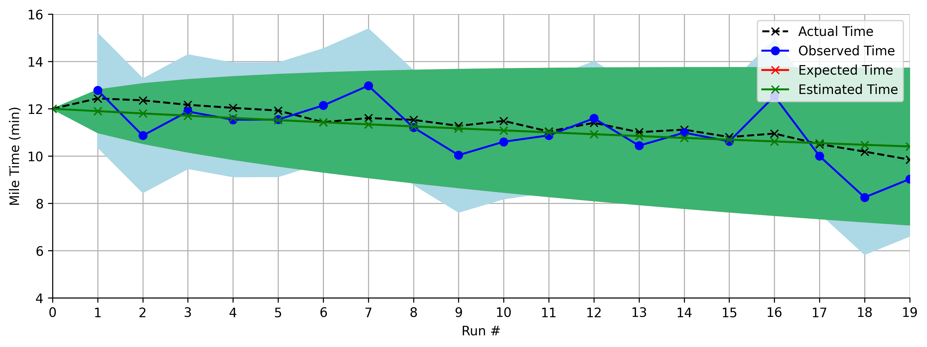
At each step, the black is the “hidden” true value, the blue is the observed time, and the green is our estimate. Initially we are very confident in our estimate, but over time the uncertainty continues to grow and grow, represented by the widening of the green region.

Now let’s see the same problem but using the gain to optimally mix the model and measurement:

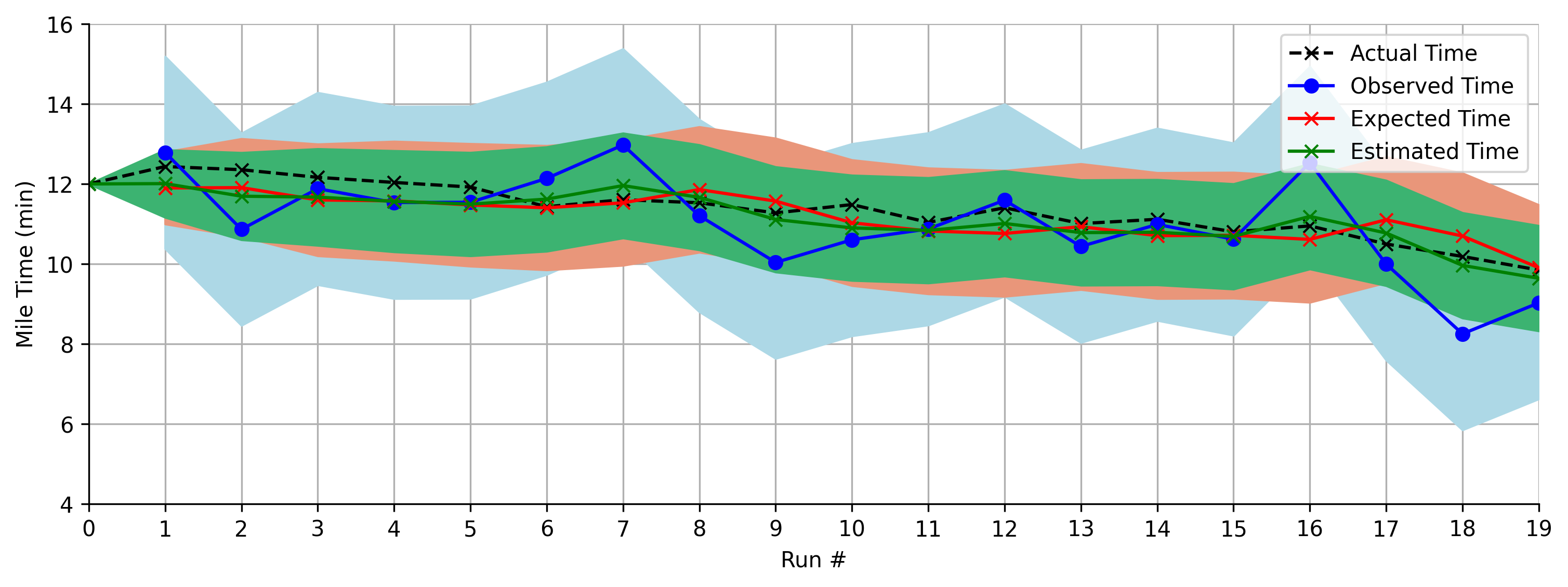
The blue is still the measurement, but now we have a red curve representing the model’s predictions separate from the final estimate. The green curve is now the result of mixing the blue and red information. Although the uncertainty in the green estimate grows initially, it eventually stabilizes as the algorithm finds the balancing point between the observation and model. Any more lean towards the observation, and the model would just end up widening the green region of uncertainty. Moving towards the observation would increase uncertainty thanks to the larger uncertainty of the measurement (blue region). Moving towards the model also increases uncertainty since we ignore the useful information provided by the measurement. By plotting the gain at each step, we can see it converge to this balancing point:

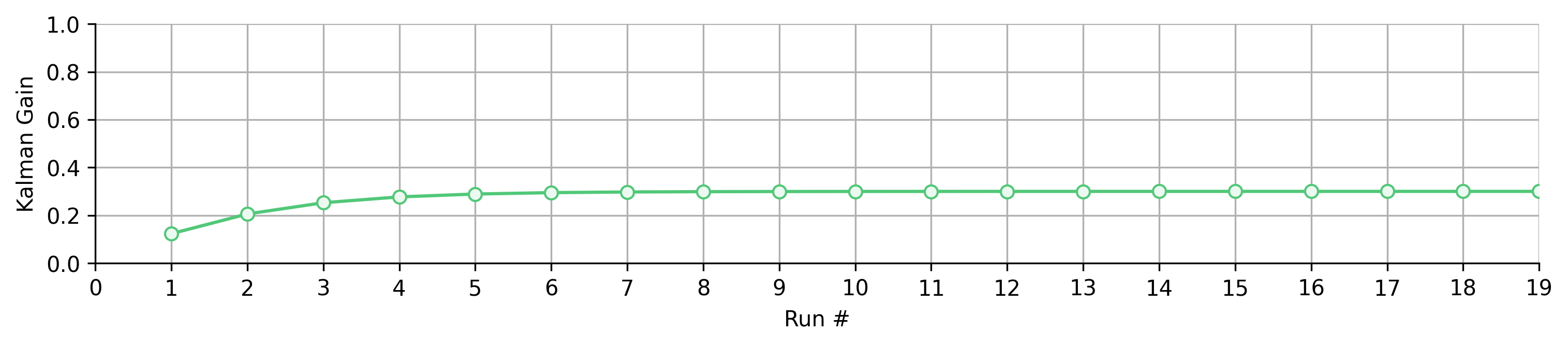
Since we start out being very confident in our model, the gain starts small—biasing the estimate towards the model’s prediction—until the uncertainty grows just enough to justify leaning more on the measurement. Then the gain flattens out.

Next lets dive into how we implement all this.

Implementing a Kalman Filter

In its basic form, here’s how we apply the Kalman filter to the mile time problem.

1. First we define the model as $\bar x_k = 0.98 \hat x_{k-1}$. This means that our model output is a 2% decrease from the previously estimated time. We also define the process variance as $\sigma_p^2 = 0.09$ and the measurement variance as $\sigma_m^2 = 0.64$. This means natural variation in the process is smaller than the variation experienced by the measurement. We don’t need to specifically define a separate measurement equation because we assume the mile time—the state—is measured directly. Also, since we know our mile time can’t decay all the way to zero, we treat the state as the mile time above seven minutes.
2. We pick the initial estimate to be $\hat x_0 = 5$ or a mile time of 5 + 7 = 12 minutes. We assume this is exactly right, so the initial estimate of the variance/squared error is just $\sigma_{\hat x_0}^2 = 0$.
3. Whenever an observation like $z_1 = 5.79$ arrives, we start by calculating the expected time using our model and previous estimate: $\bar x_1=0.98 \hat x_0 = 0.98 \cdot 5 = 4.9$
4. Next, we figure out the uncertainty/variance of this model output: $\sigma_{\bar x_1}^2 = (0.98\sigma_{\hat x_0})^2 + \sigma_p^2 = \sigma_p^2 = 0.09$
5. At this point we can calculate the gain: $k_1=\sigma_{\bar x_1}^2 / (\sigma_{\bar x_1}^2 + \sigma_m^2) = 0.12$
6. Combining the model output and actual observation, we get: $\hat x_1 = \bar x_1 + k_1 (z_1 - \bar x_1) = 4.9 + 0.12(5.79 - 4.9) = 5.01$. Adding this to our minimum time of seven minutes we get 5.01 + 7 = 12.01 minutes.
7. Finally, we update our estimate of the error: $\sigma_{\hat x_1}^2 = ((1 - k_1) \sigma_{\bar x_1})^2 + (k_1 \sigma_m)^2 = 0.08$. Notice how this error is lower than both the model and the measurement individually!

We continue to repeat steps 3 to 7 to filter the whole set of observations:

A notebook code example can be found here: kalman.ipynb

If you can bear with me for a jump from single values to matrices, we can write the general algorithm as:

1. Define constants for the state transition $\Phi$, process covariance $Q$, measurement matrix $H$, and measurement covariance $R$ using knowledge of the system.
2. Set $\hat x_0$ and $P_0$ as the initial estimate of the state and state covariance (squared error).
3. Calculate the new uncorrected estimate: $\bar x_k = \Phi \hat x_{k-1}$
4. Calculate the covariance of the uncorrected estimate: $\bar P_k = \Phi P_{k-1} \Phi^\top + Q$
5. Calculate the gain: $K_k = \bar P_kH^\top(H \bar P_k H^\top + R)^{-1}$
6. Collect measurement $z_k$
7. Correct the estimate using the measurement information: $\hat x_k = \bar x_k + K_k (z_k-H\bar x_k) = (I - K_k H)\bar x_k + K_k z_k$
8. Calculate the variance of the corrected estimate: $P_k = (I - K_kH)\bar P_k(I - K_kH)^\top + K_kRK_k^\top$
9. Repeat steps 3-8 for each time step

Of course, you may be wondering where these equations come from. How do we know these are the right steps? Time for a little lot of math…

Deriving the Kalman Filter

This derivation is heavily derived from Tutorial: The Kalman Filter. I’m not smart enough to figure it out myself.

We start by defining a model that describes how the state/system changes from one step to the next:

$$x_k = \Phi x_{k-1} + w_k \tag{1}$$

where $x_{k-1}$ is the previous state, $\Phi$ is called the state transition matrix, and $w_k$ is the white noise associated with the process. Since the state itself may be hidden, we can write a measurement equation that links the state to a sensor value we can actually observe:

$$z_k = H x_{k} + v_k \tag{2}$$

where $z_k$ is the measurement, $H$ is the observation matrix, and $v_k$ is the measurement white noise.

Our overall goal is to find a way to estimate the true state $x_k$ that minimizes the error. We define the error as:

$$e_k = x_k - \hat x_k\tag{3}$$

where $\hat x_k$ is our estimate of the state. If we ignore the white noise, we can use the state transition model to guess the state based on our previous estimate:

$$\bar x_k = \Phi \hat x_{k-1}\tag{4}$$

We can think use our sensor measurements to “correct” this estimate:

$$\begin{aligned} \hat x_k &=\bar x_k + K_k(z_k - H\bar x_k) \\ &= \bar x_k + K_k(Hx_k + v_k - H \bar x_k) \end{aligned}\tag{5}$$

where $K_k$ is a parameter that controls the correction based on the difference between the actual and observed measurements. Notice that in the last step we swapped the observation with our model of the observation from Eq. (2).

Ultimately, we want to minimize the expected value of the squared error between our final estimate and the true state as shown in Eq. (3).

This isn’t arbitrary—minimizing the squared error is equivalent to maximizing the Gaussian likelihood of the model. Of course, this assumes that the state follows a Gaussian/normal distribution.

It turns out that then mean squared error is the trace (sum of diagonal elements) of the error covariance matrix:

$$\mathbb E[e_k^2]= \text{tr}(\mathbb E[e_ke_k^\top]) = \text{tr}(P_k)$$

where we label the error covariance matrix as $P_k$. Let’s start by calculating this error covariance:

$$\begin{aligned} P_k &=\mathbb E[e_ke_k^\top] \\ &= \mathbb E[(x_k - \hat x_k)(x_k - \hat x_k)^\top] \end{aligned}\tag{7}$$

Substituting our definition of the estimate from Eq. (5) we get:

$$\begin{aligned} P_k &= \mathbb E[(x_k - \bar x - K_k(Hx_k+v_k-H\bar x_k))(x_k - \bar x - K_k(Hx_k+v_k-H\bar x_k))^\top] \\ &= \mathbb E[(x_k - \bar x - K_kHx_k - K_kv_k+K_kH\bar x_k)(x_k - \bar x - K_kHx_k-K_kv_k+K_kH\bar x_k)^\top] \\ &= \mathbb E[((I - K_kH)x_k - (I - K_kH)\bar x_k - K_kv_k)((I - K_kH)x_k - (I - K_kH)\bar x_k - K_kv_k)^\top] \\ &= \mathbb E[((I - K_kH)(x_k - \bar x_k) - K_kv_k)((I - K_kH)(x_k - \bar x_k) - K_kv_k)^\top] \end{aligned}$$

This is a mess. However, we can make a very helpful observation by looking at one of the factors (both are the same, but one is transposed):

$$(I-K_kH)(x_k-\bar x_k) - K_kv_k$$

The matrices are deterministic constants for a given step $k$, as is the initial prediction $\bar x_k$. On the otther hand, both $x_k$ and $v_k$ are both random variables as defined in Eqs. (1) and (2). The properties of a variance/covariance matrix (see Covariance matrix) tell us that

$$\text{var}(X+Y) = \text{var}(X) + \text{cov}(X, Y) + \text{cov}(Y, X) + \text{var}(Y)$$

If we let $X = (I - K_kH)(x_k - \bar x_k)$ and $Y=K_kv_k$, we can split up the variance/covariance of the error into

$$P_k = \text{var}(X - Y) = \text{var}(X) - \text{cov}(X, Y) - \text{cov}(Y, X) + \text{var}(Y)$$

Since the noise causing variation in the two random variables is white noise, we can assume that the two noise values $w_k$ and $v_k$ are not correlated with each other. This means that $\text{cov}(X, Y) = \text{cov}(Y, X) = 0$, which simplifies our expression to

$$P_k = \text{var}(X) + \text{var}(Y)$$

Inserting our definitions we then get

$$P_k = \mathbb E[((I-K_kH)(x_k - \bar x_k))((I-K_kH)(x_k - \bar x_k))^\top] + \mathbb E[(K_kv_k)(K_kv_k)^\top]$$

We can distribute the transpose and then remove the constants from the expectations:

$$\begin{aligned} P_k &= \mathbb E[(I - K_kH)(x_k - \bar x_k)(x_k - \bar x_k)^\top(I - K_kH)^\top] + \mathbb E[K_k v_k v_k^\top K_k^\top] \\ &= (I - K_kH)\mathbb E[(x_k - \bar x_k)(x_k - \bar x_k)^\top](I - K_kH)^\top + K_k \mathbb E[v_k v_k^\top ]K_k^\top \end{aligned}$$

If we define the measurement noise variance as

$$R = \mathbb E[v_kv_k^\top]\tag{8}$$

and the variance of the initial error $\bar e_k = x_k - \bar x_k$ as

$$\bar P_k = \mathbb E[\bar e_k \bar e_k^\top]\tag{9}$$

we can further simplify to get

$$P_k = (I - K_kH)\bar P_k(I - K_kH)^\top + K_k RK_k^\top$$

Returning to our goal, we want to minimize the trace of this matrix. We can make things a little easier by first expanding our equation for $P_k$:

$$\begin{aligned} P_k &= (I - K_kH)\bar P_k(I - K_kH)^\top + K_k RK_k^\top \\ &= (\bar P_k - K_kH\bar P_k)(I - K_kH)^\top + K_k R K_k^\top \\ &= \bar P_k - K_kH\bar P_k - \bar P_k H^\top K_k^\top + K_kH\bar P_k H^\top K_k^\top + K_kRK_k^\top \\ &= \bar P_k - K_kH\bar P_k - \bar P_k H^\top K_k^\top + K_k(H\bar P_k H^\top + R)K_k^\top \end{aligned}$$

Applying the trace with properties shown in Trace (linear algebra), we get

$$\text{tr}(P_k) = \text{tr}(\bar P_k) - 2 \text{tr}(K_k H \bar P_K) + \text{tr}(K_k(H\bar P_k H^\top + R)K_k^\top)$$

We can minimize with respect to our free parameter $K_k$ by finding the critical point where the derivative of the trace with respect $K_k$ is zero (see Properties of the Trace and Matrix Derivatives):

$$\frac{d\text{tr}(P_k)}{dK_k} = - 2 (H \bar P_K)^\top + 2 K_k (H\bar P_k H^\top + R) = 0$$

Rearranging this equation gives us:

$$\begin{aligned} 2 (H \bar P_K)^\top &= 2 K_k (H\bar P_k H^\top + R) \\ (H \bar P_K)^\top &= K_k (H\bar P_k H^\top + R) \\ \implies K_k &= (H \bar P_K)^\top (H\bar P_k H^\top + R)^{-1} \\ &= \bar P_k H^\top (H\bar P_k H^\top + R)^{-1} \end{aligned}\tag{10}$$

where the last step comes from knowing that $\bar P_k$ is symmetric. Roughly speaking, the final line of Eq. (10) shows that $K_k$ shrinks as the measurement variance $R$ grows. Intuitively, this means that as the uncertainty around the measurement grows, we down weight the measurement-based correction factor in Eq. (5). However, if $\bar P_k$ —the uncertainty around our initial guess $\bar x_k$—grows, so will $K_k$. This means that as we become less sure about our guess, we lean more heavily on the information from the measurement in Eq. (5).

We still need one more piece of information. What actually is $\bar P_k$? Let’s return to its definition:

$$\bar P_k \triangleq \mathbb E[(x_k - \bar x_k)(x_k - \bar x_k)^\top] = \text{var}(x_k - \bar x_k)$$

Substituting our definition of $x_k$ from Eq. (1) and $\bar x_k$ from Eq. (4) we see

$$\begin{aligned} \bar P_k &= \text{var}(x_k - \bar x_k) \\ &= \text{var}(\Phi x_{k-1} + w_k - \Phi \hat x_{k-1}) \\ &= \text{var}(\Phi(x_{k-1} - \hat x_{k-1}) + w_k) \\ &= \text{var}(\Phi(x_{k-1} - \hat x_{k-1})) + \text{var}(w_k) \\ &= \Phi\text{var}(x_{k-1} - \hat x_{k-1})\Phi^\top + \text{var}(w_k) \end{aligned}$$

Swapping in the definitions of variance we get

$$\begin{aligned} \bar P_k &= \Phi \mathbb E[(x_{k-1} - \hat x_{k-1})(x_{k-1} - \hat x_{k-1})^\top]\Phi^\top + \mathbb E[w_kw_k^\top] \\ &= \Phi \mathbb E[e_{k-1}e_{k-1}^\top]\Phi^\top + \mathbb E[w_k w_k^\top] \end{aligned}$$

Notice that $\mathbb E[e_{k-1}e_{k-1}^\top] = P_{k-1}$ from our definition in Eq. (9). If we let $Q = \mathbb E[w_kw_k^\top]$ be the variance of the process noise from Eq. (1), we can write

$$\bar P_k = \Phi P_{k-1}\Phi^\top + Q\tag{11}$$

Phew, we made it! If you go back to the end of the last section, you’ll find all these equations form the steps of the matrix-based Kalman algorithm!